There is no universal price for running a fan all day. The useful answer comes from three project-specific inputs: the fan system’s average real electrical input, the number of hours it actually operates, and the energy rate that applies during those hours. Nameplate power and a headline electricity price can produce a quick estimate, but they often describe the wrong boundary.
This guide shows how to build a number you can audit. It also explains when a simple kilowatt-hour calculation is enough, when operating modes must be separated, and why a commercial bill may contain charges that should not be assigned wholesale to one fan.
Use the basic fan running-cost formula
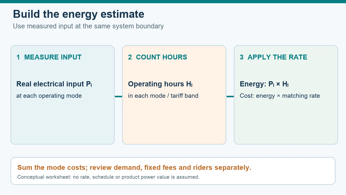
Start with energy, not currency. If P is average real input power in kilowatts and H is operating time in hours, then energy use is E = P × H in kilowatt-hours. Multiply that result by the applicable energy rate R to estimate the variable energy charge: Cost = P × H × R.
Keep units visible while you work. Convert watts to kilowatts by dividing by 1,000. A fan that truly runs without interruption operates for 24 hours per day, 720 hours in a 30-day period, and 8,760 hours in a 365-day year. Planned shutdowns, cycling and setback schedules reduce operating hours; speed control changes the power assigned to those hours.
Choose the right power value
The most important input is usually P. Use average real electrical input power at the boundary you intend to cost. Motor output power, maximum input, rated input and measured system input are different quantities. A maximum rating is useful for electrical design, but it is not automatically the average draw across a month.
Define what the measurement includes. Depending on the installation, the boundary may include an integrated EC drive, an external VFD, a transformer, controls and standby consumption. Do not compare one option at the motor terminals with another at the incoming supply. For more context on system boundaries and duty points, see Longwell’s HVAC fan efficiency and system-design guide.
Calculate variable-speed and cycled operation
A single average power figure is convenient only when it is representative. If the fan has distinct modes, calculate each one separately: E = Σ(Pi × Hi). Add the energy for full-load operation, reduced-speed operation, standby and any scheduled off time over the same billing period.
For an existing installation, a compatible energy meter or building-management trend can give a stronger input than a guessed load factor. Cumulative kilowatt-hours over a representative period are especially useful because they already capture changing modes. A plug-in meter may be suitable for a compatible single-phase load; hard-wired or three-phase measurements should be planned and performed by qualified personnel. This article is a costing method, not a live-electrical-work procedure.
Match the rate to the hours
Electricity rates vary by region, customer class, season, time of use, consumption tier, currency and effective date. Record those details next to the calculation. When the future rate is uncertain, use low, base and high scenarios rather than hiding uncertainty inside one precise-looking total.
If the fan runs across several time-of-use bands, pair each block of energy with its own rate, then add the results. Do not assume that the average price obtained by dividing the entire bill by total kilowatt-hours is the price of the next kilowatt-hour. That bill-wide average may include fixed charges and other items that do not move in direct proportion to the fan’s energy use.
Separate energy, demand and fixed bill items
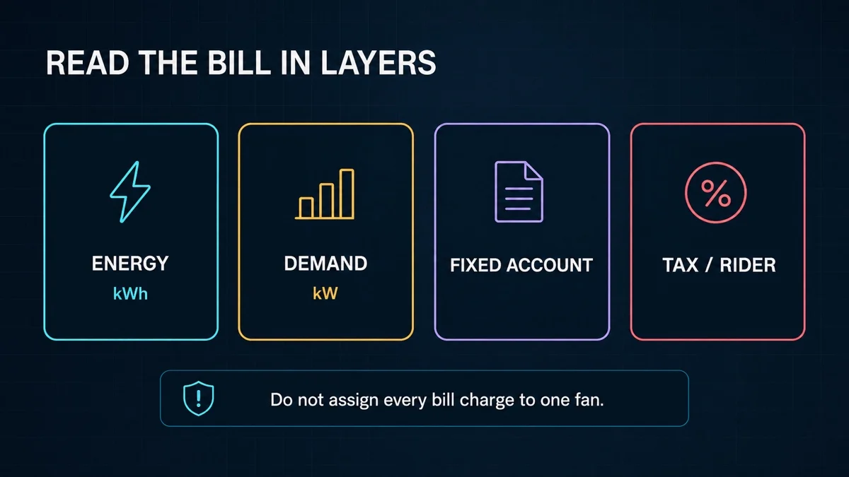
An energy charge is normally tied to kilowatt-hours. Some commercial tariffs also include a demand charge based on a measured kilowatt peak during a defined interval. A fan affects that charge only if its operation changes the applicable peak under the tariff rules. Fixed account fees usually remain even when the fan is off, so assigning the entire fee to one fan would overstate its cost.
Taxes, riders and adjustments may be percentage-based, energy-based, demand-based or fixed. Read the tariff rather than assuming a single multiplier. For a budget estimate, state which items are included and which are excluded; for an investment decision, have the site’s billing structure checked by the person responsible for utility accounts.
Compare fans at the same useful duty
A lower wattage label does not prove lower operating cost if the fans are doing different jobs. Compare candidates at the same required airflow and pressure, with the same air density, inlet and outlet conditions, filter state, control strategy and measurement boundary. The operating point belongs to the assembled system, not to a catalog maximum.
If the task is still being defined, the fan airflow, static-pressure and efficiency guide explains why free-air flow alone is not enough. After the duty is known, Longwell’s EC backward-curved fan family provides a category-level screening path; final selection still requires the current curve, drawing and electrical data for the exact model.
Treat fan-law savings as a scenario
The fan affinity laws can help explore how a speed change may affect flow, pressure and power under similar conditions. They are not a substitute for the actual fan curve, system curve or measured input. Static-pressure components, drive efficiency, control losses and a shifted operating point can all move the real result away from a simple cube-law estimate.
Use the laws to create a testable scenario, then confirm the proposed operating point and input power. Any savings calculation should compare the same useful duty and load profile. A label-only comparison can otherwise reward a fan that consumes less power simply because it delivers less of the required airflow or pressure.
Build an estimate someone else can reproduce
A practical worksheet should show the measurement boundary, power source, operating modes, hours, rate source, currency, effective date, bill components, calculation and exclusions. Keep more precision in the intermediate steps than in the final answer, then round the result to match the uncertainty in the inputs.
For a new design, calculate low, base and high operating scenarios. For an existing system, compare the estimate with a representative meter interval and the corresponding bill period. The goal is not a universally impressive number. It is a transparent operating-cost range that another engineer or buyer can recalculate when the duty, schedule or tariff changes.